Layer functionalities
Filters
Description
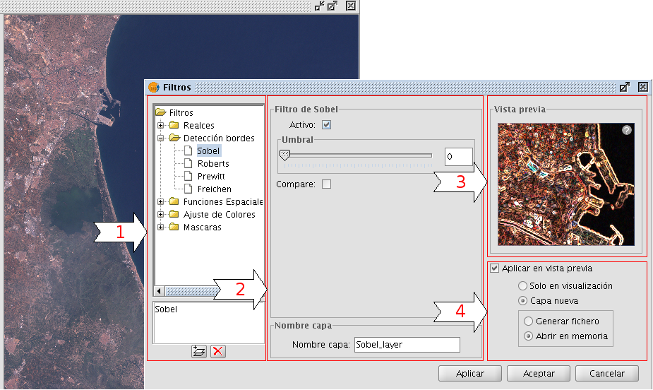
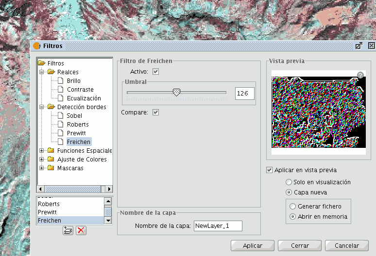
Filtering is a process by which we can enhance images. gvSIG can filter images through a variety of filtering methods. In the upper left part of the Filter dialog, the filters are grouped by type (1). By double-clicking one of the filters or by clicking on the "Add Filter" button on the bottom left, the filter will be added to the list of filters in the lower left part of the Filter dialog. All filters in the filter list will be applied in the preview. If you want to remove a filter from the list, you can either double-click on the filter or click on the "Delete filter" button. The filters in the list will be applied to the image in the order that they appear. Keep in mind that the order in which the filters are applied will affect the result, and changing the order of the filters may change the output.
In the middle of the dialog window are the controls of the selected filter (2). When changing the controls of one of the filters from the filter list, the results will be directly shown in the preview window. Below the middle part of the dialog you can change the name of the output layer that will be generated when clicking "Apply" or "Close".
On the right side of the dialog you can preview the outcome of the filters (3). (See documentation on "Preview tool"). In the lower right part you can select whether you want to display the filters over the selected layer or save the filtered image as a new layer (4).
The button "Apply" will apply the changes according to the entered parameters, keeping the Filter dialog open. The "Close" button will apply the changes and close the Filter dialog. The "Cancel" button will close the Filter dialog without applying any filters.
All filters in the filter list can be activated or de-activated through the "Active" checkbox. This checkbox is usually located in the upper part of the filter control panel.
Configuration panel for the image filters
Generate a new layer or apply to current layer
The number of applied filters will affect the time that it will take to draw the layer. If you choose to apply the filters to the current layer, the drawing and re-drawing of the layer may slow down while the filters are applied. If the filter results are saved as a new layer, the filtering process has to be done only once so that the next time the layer is drawn, it will not be slowed down by the filtering. Therefore, it is generally recommended to save the output to a new layer if possible. There are cases though in which it is not recommended to generate a new layer. For example, if you have a large orthophoto and you only want to change the brightness a little, it could take more time to save the output as a new layer. If the brightness filter is applied over the current view, the area on which the filter is applied is much smaller which makes the drawing faster. It is up to the user to decide whether it is better to create a new layer or display the filters on the view of the current layer.
Enhancements
The brightness filter changes the brightness value of the layer. You can increase or decrease the brightness by moving the position of the sliding bar or by entering the value directly in the text box and press enter.
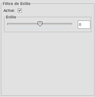
Brightness filter
The contrast filter changes the contrast value of the layer. You can increase or decrease the contrast by moving the position of the sliding bar or by entering the value directly in the text box and press enter.
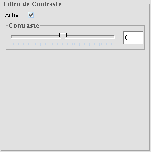
Contrast filter
Spatial filters
With this type of filter, graphical transformations like smoothing, edge detection, sharpening etc. are applied to the image.
The following filter types can be applied:
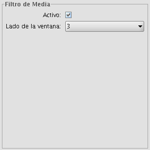
MEDIAN FILTER
The median filter applies a kernel of a certain size, which is determined by the user through the sliding bar labeled Window side.
The median filter is normally used to smoothen and to reduce noise in an image, by moving a kernel of N x N number of pixels over the image and evaluating each central pixel, replacing its value with the median of its neighboring pixels. Compared to the Mean filter, the advantage of the Median filter is that the final pixel value is a value that actually occurs in the image and not an average.
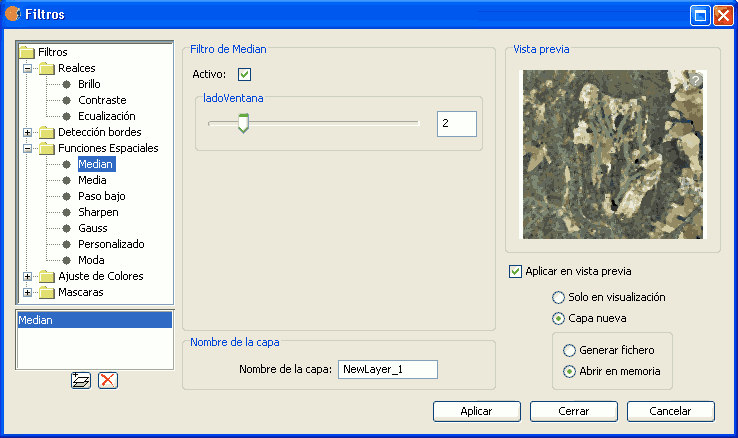
Median filter
MEAN FILTER
The mean filter applies a kernel of a certain size, which is determined by the user through the sliding bar labeled Window side.
The filter replaces the value of the central pixel with the mean value of the surrounding pixels. Each value of the kernel would be one and the divider would be the total number of elements in the kernel (i.e. a kernel of 3 x 3 would replace the value of the central pixel by the average value of the nine pixels covered by the kernel).
Mean filter
LOW PASS FILTER (smoothing filter)
The low pass filter applies a kernel of a certain size, which is determined by the user through the sliding bar labeled Window side.
Using a low pass filter tends to retain the low frequency information within an image while reducing the high frequency information.
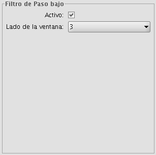
Low pass filter
SHARPENING FILTER
By moving the slider to change the sharpness (values from 1-100), the contrast of an image can be changed. The results can be evaluated in the preview window. With a higher contrast, details in the image can be accentuated but the noise will also increase.
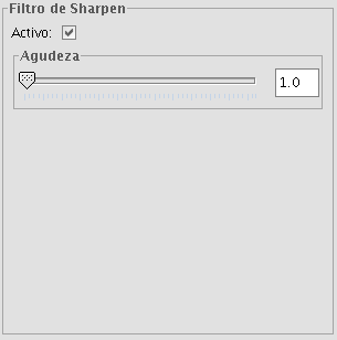
Sharpening filter
GAUSS FILTER
The Gauss filter applies a kernel of a certain size, which is determined by the user through the sliding bar labeled Window side.
The maximum value appears in the central pixel and gradually decreases for pixels that are further away from the central pixel.
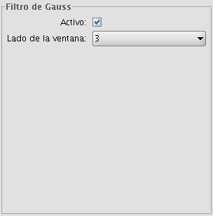
Gauss filter
CUSTOM FILTER
This is a kernel of 5 x 5 or 3 x 3, for which the values can be introduced by the user. After multiplying the pixel values with the kernel values, the result will be divided by the number specified in the Divisor textbox.
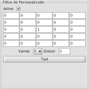
Custom filter
MODE FILTER
The mode filter applies a kernel of a certain size, which is determined by the user through the sliding bar labeled Window side.
This filter takes the value that occurs most in the surrounding pixels and assigns it to the central pixel.
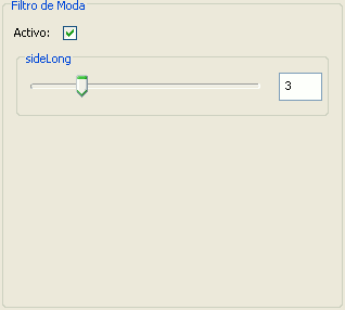
Moda filter
Colour adjustment
Adjustment of RGB values
It is possible to change the balance between Red, Green and Blue in an image if needed. To do this, move the sliding bar to increase or decrease the values or enter the value directly in the text box next to the sliding bar. Ticking the "Brightness" check box ensures that the brightness level of the pixels will be maintained while the RGB values are changed.
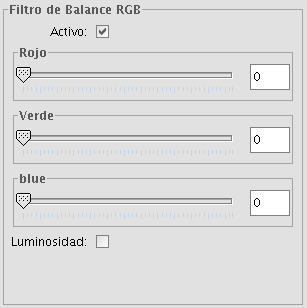
RGB balance filter
Adjustment of CMY values
It is possible to change the balance of Cyan, Magenta and Yellow in an image if needed. To do this, move the sliding bar to increase or decrease the values or enter the value directly in the text box next to the sliding bar. Ticking the "Brightness" check box ensures that the brightness level of the pixels will be maintained while the CMY values are changed.
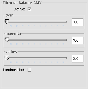
CMY balance filter
Adjustment of HBS values
It is possible to change the balance of Hue, Brightness and Saturation in an image if needed. To do this, move the sliding bar to increase or decrease the values or enter the value directly in the text box next to the sliding bar.
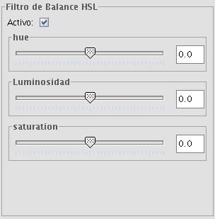
HBS balance filter
Edge detection
These filters attempt, through the use of kernels, to detect edges in the image and change the image so that these edges are enhanced, while the rest of the image is grayed out.
Filter dialog. Edge detection
There are four edge detection filters, all with the same interface and options, in which the user chooses a threshold in the range 0-255, and the possibility compare the results by ticking the compare check box:
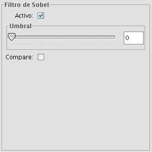
Sobel filter example
SOBEL
The Sobel filter detects the horizontal and vertical edges separately on a grayscale image. Colour images are converted to RGB gradations. The result is a transparent image with black lines and some remains of colour.
ROBERTS
The Roberts filter is suitable for detecting diagonal edges. It offers good performance in terms of location. The major drawback of this filter is its extreme sensitivity to noise and therefore has poor detection qualities.
PREWITT
The Prewit filter detects edges in all directions as it consists of 8 kernels that are applied over the image pixel by pixel.
FREI-CHEN
The Frei-Chen filter processes the neighbouring pixels as a function of their distance from the pixel that is being evaluated. The result is that edges in all directions are detected.
Masks
Transparent area
With this functionality it is possible to set the transparency level of a Region of Interest (ROI). The region of interest must have been defined previously. If the layer does not have a region of interest, the following message will appear: "A Region of Interest (ROI) must be defined for this layer to apply this filter. Please go to the dialog Area of Interest and select at least one ROI." If there are already one or more ROI associated with the layer, the message will not appear. Instead, a list of ROI will be shown, from which you can select one or more by ticking the corresponding check box. Then, adjust the level of transparency with the slide bar or by entering the value directly in the text box next to the slider. Ticking the check box labeled as "Inverse" will result in the opposite effect; all of the image except for the ROI will be set to the specified transparency level.
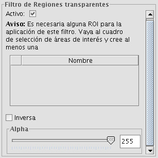
Transparent area filter
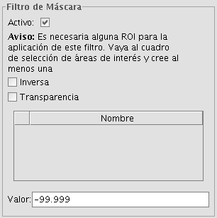
Mask
With this functionality it is possible to cut out a Region of Interest (ROI) that has been previously defined for the layer by assigning a fixed user-specified value to the rest of the image outside the ROI. If the layer does not have a region of interest, the following message will appear: "A Region of Interest (ROI) must be defined for this layer to apply this filter. Please go to the dialog Area of Interest and select at least one ROI." If there are already one or more ROI associated with the layer, the message will not appear. Instead, a list of ROI will be shown, from which you can select one or more by ticking the corresponding check box. Then, select the value to be assigned to the pixels outside the ROI by typing a number in the "value" text box. The default value is -99,999. Ticking the check box labeled as "Inverse" will result in the opposite effect; the ROI will be assigned the specified value while the rest of the image values are maintained.
Mask filter
Histogram
Description
To launch the histogram dialog window, use the drop-down toolbar selecting the "Raster Layer" button on the left and "Histogram" in the drop-down button on the right. Make sure that the text box that displays the current layer is set to the name of the raster layer for which you want to see the histogram.

Histogram icon
The Histogram dialog shows a histogram of the statistical distribution of pixel values in the current view. This information is often useful when you are trying to color balance an image. In the middle of the dialog you will see the graph on which you can right-click to show a context menu with general options for this kind of graphics.
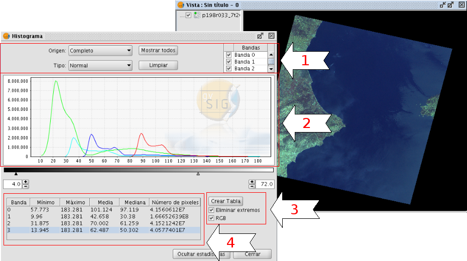
Histogram dialog window
In the upper part of the dialog (1) are the controls to configure the histogram:
1. Type of histogram
There are three types: "Normal", "Accumulated" and "Logarithmic".
- Normal: This is the normal histogram in which for every pixel value on the X axis the number of pixels is shown on the Y axis.
- Accumulated: Shows the accumulated number of pixels for every pixel value. The graph is therefore ascending.
- Logarithmic: Displays the histogram on a logarithmic Y axis, which may be useful for images that contain substantial areas of a constant value.
2. Data source
With this option you can select the data source for the histogram:
Current view (R,G,B):
With this option, the pixel values that are displayed in the current view of gvSIG will be used for the histogram. Therefore, the band selector shows only the R, G, and B values which are the visual bands. Every band will appear in its corresponding colour in the graph (red for R, green for G and blue for B). This is the default option when the histogram dialog is opened.
Complete histogram:
With this option, the histogram for the whole raster layer is calculated. Because of the amount of time that it would take to calculate the histogram for large images, the histogram is only calculated once and saved with a .rmf extension in the directory in which the image is stored. After the first time, the histogram for the same layer can be displayed much faster. (Keep in mind that if you delete the .rmf file that is stored with the image, you will lose its histogram information.)
3. Band selection
Apart from identifying to which band each histogram corresponds through its colour (in case of the current view Data Source) you can also identify the band by hovering the mouse over a point in the graph. The tooltip displays the band name and the value of the point.
Zoom operations
We can zoom in and out of the graph using the mouse.
- To zoom in on a part of the graph, draw a rectangle over it by pressing and dragging the mouse.
- To return to the original graph, click on the left mouse button on any point in the graph and drag to the left, then release the mouse button.
You can also zoom in and out using the context menu.
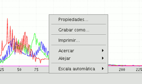
Context menu
When you right-click on any part of the graph, the context menu is shown with the following options:
Histogram options. Context menu
- Properties: This will open the properties dialog of the graph, where you can configure characteristics such as the background colour, title, font etc.
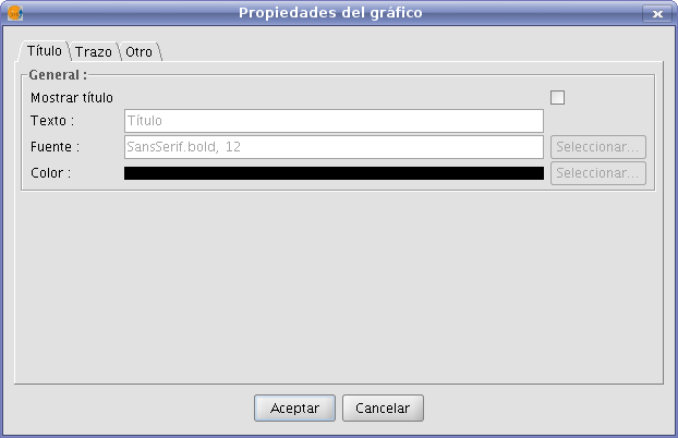
Histogram properties
- Save As: to save the graph as an image.
- Print: this opens the printer dialog from where you can print the graph.
- Zoom In: to zoom in on one or both of the axes.
- Zoom Out: to zoom out on one or both of the axes
- Auto Range: to adjust the zoom automatically to the window size, for one axis or for both.
5. Statistics (4)
The controls that appear under the graph allow the user to restrict the range of values (X axis of the histogram) on which the histogram is based. The default setting is the complete range so that, for example in a Byte data type image, the statistics are calculated for all the pixel values from 0 to 255. You can enter the values directly in the text boxes or use the + and – controls next to the text boxes. You can also slide the triangles over the sliding bar to select the range of values.

Sliding bar with pixel ranges
In this table, the statistics that correspond to the selected range of pixel values are shown in the text boxes. Each row of the table corresponds to one raster band as displayed in the histogram. The columns that are shown are:
- Minimum pixel value for the selected interval.
- Maximum pixel value for the selected interval.
- The mean (average) of all the pixel values for the selected interval in the histogram.
- Median pixel value for this interval.
- The number of pixels included in the selected interval.
6. Export the table (3)
You can export the table through the option "Save as DBF". The data contained in this table are the values of the current histogram. After creating the DBF table, it can be used as any other table in gvSIG.
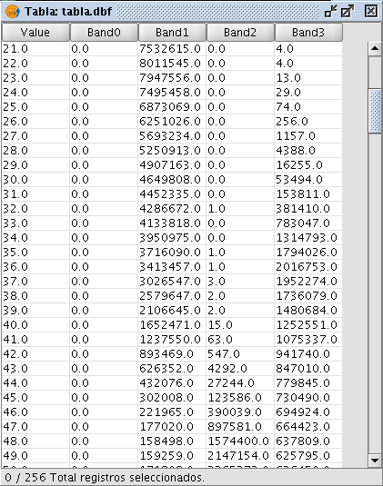
Resulting DBF table
Preferences
The Raster section of the Preferences dialog contains the option "Number of classes" where you can set the number of intervals in which the histogram is divided when the data type of the image is not Byte. For Byte images, this value is 256. In the preferences dialog, the default value of this option is 64 but you can choose any of the options (32, 64, 128, and 256). The intervals are the parts in which the range of values is divided. For example, if we have a DTM with values between 0 and 1 and there are 64 intervals, each interval will have a range of 1/64.
The number of classes does not only refer to histograms but also to other functionalities that require a division in intervals of value ranges.
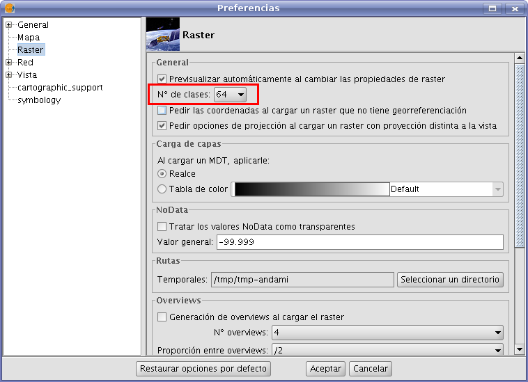
Raster Preferences
Radiometric enhancement
The maps that are obtained through digital processing of satellite imagery are useful not only for thematic mapping, but also as a backdrop on which map features can be overlaid. If the visible bands are displayed in a colour composition through the colouring of each band with the corresponding colour gun, it is important that the bands are sufficiently enhanced so that the colours appear more natural. The final display colour depends not only on the direct result of the chosen colour composition but also on the radiometric post-processing. The satellite image map will be more useful as backdrop if the bands are enhanced and displayed in colours that match the natural colours as the human eye perceives them. gvSIG provides the enhancement tools to adjust the colours for each band.
In the following sections the different parts of the dialog are described:
Histograms
The central part shows two graphs (1). The graph on the left is the histogram of the input image. The graph on the right shows the histogram of the output image. The graphs that are presented with a yellow line can be modified with the mouse. When you change the input histogram, the output histogram will be changed accordingly and you can preview the result.
In the upper corners of the input histogram are the maximum and minimum values of the raster displayed. In the lower corners, the maximum and minimum values that are being included in the enhancement are displayed. The percentage of values that are being left out of the histogram appears in parentheses. These values can be modified by grabbing and dragging the dotted vertical lines on the side of the graph. Dragging the left line will modify the minimum value, while dragging the right line will modify the maximum value. (This way, by leaving out the values that are not used in the input image, you can stretch the output values over the whole range of available values, so that the visual quality is improved.)
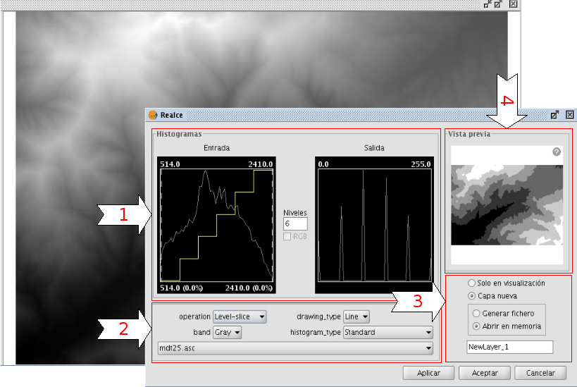
Radiometric Enhancement dialog
Controls
In the lower part of the dialog (2) you will find some controls with the following options:
Type of function:
The enhancements will replace each input value with an output value. This process is done by creating a look-up table which provides the correspondence between a range of input data and a range of output data. To apply this correspondence, a fuction is used. The used function and its parameters are chosen by the user.
Linear enhancement
- Linear: Linear enhancements apply the correspondence between the input data and output data in a linear way. In the simplest case, a straight line will correlate each value in the input interval with the corresponding value in the output interval in a complete equidistant way. For example, if you have an output range between 0 and 255 and the input values are between 0 and 1, the input value 0.5 would result in an output value of 127.5. This is the default algorithm when you first open the radiometric enhancement dialog. Variations of this algorithm can be achieved by introducing break points in the yellow line, by clicking on the line at the point where you want to break it. You can remove break points by right-clicking on them. Existing break points can be moved by dragging them. The effect is that the linear filter is divided in parts with different inclination, so that different parts will follow a different linear function as defined by the inclination of the corresponding line part.
Linear radiometric enhancement
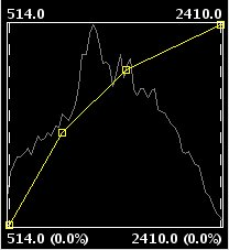
- Level slice (piecewise linear): This is a type of linear enhancement. It divides the function stepwise in equidistant parts. The effect is that the input values between two points on the same horizontal level will be assigned the same output values, so that the resulting image will have colour intervals without transitions. (This may be useful to highlight a specific range of gray levels in an image, for example to enhance certain features.) You can modify the number of intervals by changing the value in the text box labeled "Levels". The default value is 6 levels.
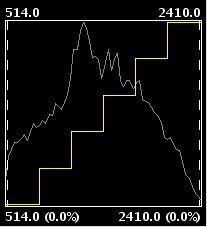
Piecewise linear enhancement
Non-linear enhancement
The non-linear enhancements have the same approach as the linear enhancements in the sense that each input value is replaced by an output value. The difference lays in the function that is assigned to produce the output values, which is non-linear. The available non-linear functions are logarithmic, exponential and square root. With each function you can modify the curve to smooth or accentuate the enhancement result.
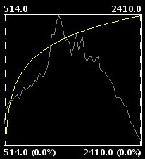
Exponential radiometric enhancement
Band
With this option you can specify the raster band to which the enhancements are applied. For a correct balance of the image, it is recommended to enhance each band separately.
Drawing type
With the option drawing type, different types of histograms can be chosen. Filled will draw a filled histogram while Line will only show the contours of the histogram. The colour of the line or fill pattern depends on the selected band. The bands Red, Green, Blue and Gray are displayed in red, green, blue and gray respectively.
Type of histogram
- Standard: Standard display of the histogram. For each possible value on the X axis, the number of pixels that are assigned this value in the output image are shown on the Y axis.
- Cumulative: For each possible pixel value on the X axis, the number of pixels that are assigned this value in the output image are shown on the Y axis. Furthermore, the number of pixels with the same or lower value are added to the result.
- Logarithmic: This shows the logarithmic value of the histogram in each position, resulting in a more balanced histogram without dominating peak values.
- Cumulative Logarithmic: This shows a cumulative histogram in logarithmic values.
RGB Check box
When check box labelled as RGB is ticked, it is assumed that the image is displayed as RGB with Byte data type and values between 0 and 255. If the checkbox is not ticked, it is assumed that the range of values are Byte data type values between -127 and 128, which will produce significant differences in the display and in the minimum and maximum values that are shown in the bottom of the input graph.
Display enhancement results
In the lower right part of the dialog (3), you can indicate how you want to see the enhancement results; in the current view or saved as a new layer.
Preview
The preview window (4) shows the real-time results of each enhancement that is applied to the image.
Save View as image
The tool for exporting the view as an image can be accessed from the drop-down toolbar by selecting "Export to raster" on the left button and "Save view to georeferenced raster" on the right button. Make sure that the name of the raster layer that you want to export is set as the current layer in the text box.

Export to raster. Save view to georeferenced raster
A message will appear to inform that you can use the selection tool to set the area in the view to export.
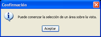
You can begin to select a area on the view
Now, you can select two points in the view to define the rectangle of the area to be exported, by clicking the first point and dragging the mouse towards the second point, then release.
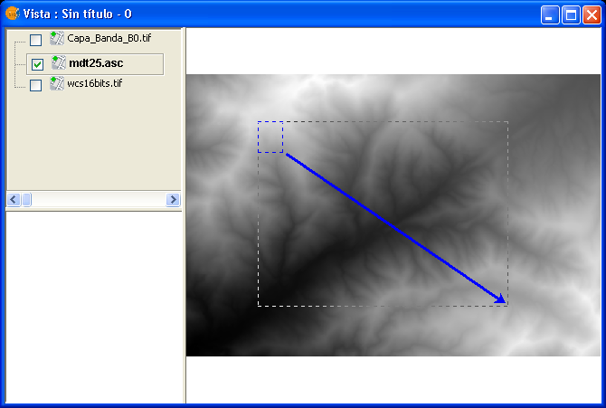
Selection of a rectangle to define the output image
Then, the Save view to georeferenced raster dialog will appear. If the selected area is too small, the dialog will not appear and a bigger rectangle must be selected.
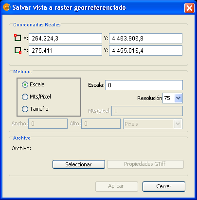
Save view to georeferenced raster dialog
The upper part of the Save view to georeferenced raster dialog shows the coordinates of the two points that define the selected area in the view. You can edit the coordinates to change the selected area.
In the option box in the central part of the dialog you can choose from three selection methods:
- Scale. Selecting this option will enable the Scale textbox and the pull-down box "Spatial resolution" which refers to the resolution in points per pixel (ppp) of the exported image. When entering a value in the Scale textbox and clicking enter, the values "Mts/pixel" and the size (Width and Height) will be recalculated for the output image.
- Mts/pixel (Meters per pixel): When selecting this option, the "Mts/Pixel" textbox is enabled. When you enter a value in the Mts/Pixel textbox and press enter, the values for "Scale" and size ("Width" and "Height") will be recalculated automatically for the output image.
- Size: When selecting this option, the text boxes to enter the "Width" and "Height" will be enabled. When you enter one of these values, the other will be calculated automatically to preserve the right proportions of the image. The other data ("Mtx/Pixel" and "Scale") will also be recalculated automatically. By default, the Width and Height values are displayed in Pixels, but you can select the units (Pixels, Cms, Mms, Mts, or Inches) in which you want to see these values.
NOTE: To save time and memory the maximum size of output images is limited to 20000 x 20000 pixels. If the intended output image is larger and you click on "Apply", gvSIG will display a message that the parameters must be changed before trying again.
Clicking the "Selection" button will open a file browser dialog where you can specify the output file. Depending on the type of file, the corresponding driver will be loaded (you will notice that the button on the right of the "Selection" button will change). For example, an output file .jp2 will open the properties dialog for Jpeg2000. The formats in which you can save are .TIF, .IMG, .BMP, .PGM, .PPM, .MPL, .RST, .JP2, .JPG, and .PNG. Furthermore but only on Linux kernel 2.4 you can also select ECW.
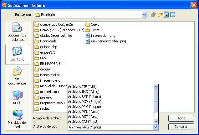
File browser dialog to save the output image
When you select the output file, the Properties button will be enabled.
For example, for geoTiff the dialog will look like this:
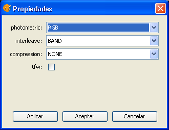
Properties geoTiff
- Photometric: [MINISBLACK | MINISWHITE | RGB | CMYK | YCBCR | CIELAB | ICCLAB | ITULAB]. This assigns the photometric interpretation. The default is RGB, as the input image consists of 3 bands of the Byte data type.
- Interleave: [BAND | PIXEL]. By default, tiff files are interleaved by band. Some applications only support interleaved by pixel, in which case you can change this option.
- Compression: [LZW | PACKBITS | DEFLATE | NONE] This refers to the data compression. The default option is NONE.
When the output image is selected and the properties set, you can click on "Apply". A progress bar will appear. Depending on the size of the output file, this process may take while. Processing times may vary between a few seconds or several days, so it is important to check the size of the output image in pixels before clicking "Apply". When finished, a screen with statistics will appear that indicates the path of the output image, the disk size, the duration of the process and whether it was compressed. To check the georeferencing of the output image, you can add it to the view as a new layer with transparency.
Clipping layers
(The clipping tool can be accessed from the raster toolbar by selecting "export to raster" from the left drop-down button and "Clipping" from the drop-down button on the right. Make sure that the raster layer that you want to clip is set as the current layer in the text box.)
With the clipping tool, you can create new layers from an existing one. The options are:
- Extract an area from the input image to be saved as a new layer (cropping)
- Modify the resolution through various interpolation methods
- Modify the order or the number of bands
- Separate the bands into multiple files
Selection of the clipping area
In the "Coordinates" tab of the clipping dialog, there are text boxes to enter coordinates. In the upper part are the values in pixel coordinates and in the lower part the real coordinates. For each item, the two upper text boxes correspond to the coordinates of the upper left corner, while the lower two text boxes correspond to the lower right corner. When changing the pixel coordinates, the real coordinates are re-calculated automatically and vice versa.
There are 3 selection methods that will fill the coordinates automatically. These methods can be activated by clicking the buttons on the bottom of the clipping dialog. From right to left, the buttons are:
- "Select from the view". This is the most commonly used tool to clip a layer. After clicking this button you can draw a rectangle over the view to select the portion of the input layer to be saved as a new layer.
- "Full Extent of the raster layer" When clicking this button, the coordinates of the upper left and lower right corner of the input image are filled in the text boxes.
- "Fit to the maximum extent of the ROIs of the layer". When clicking this button, the extent of the area covered by the ROIs associated with the layer is calculated, and the coordinates are filled in the text boxes.
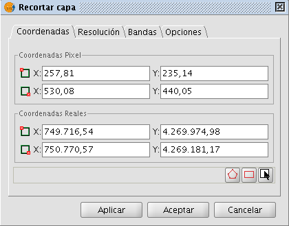
Clipping dialog. Coordinates tab
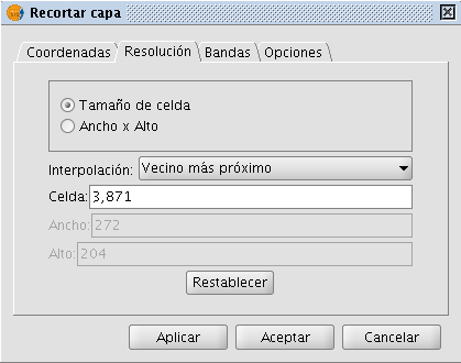
Modifying the resolution
In the "Spatial resolution" tab of the Clipping dialog, you can modify the resolution of an output image through various interpolation methods. There are two option boxes located on the upper part of this tab:
- Cell size: Ticking this option will activate the text box labeled "Cell", where you can introduce the new cell size value. By default, the text box shows the cell size of the input image.
- Width x Height: Ticking this option will activate the text boxes labeled "Width" and "Height" where you can introduce the desired width and height of the output image. When changing the width, the height will be re-calculated automatically and vice versa to maintain the correct proportions of the selected area.
When modifying the resolution it is necessary to resample and re-assign the pixel values for the output image through an interpolation method. There are four interpolation methods available: Nearest neighbour, Bilinear, inverse distance and B-Spline. The nearest neighbor is the fastest interpolation method, but the results in pixilation of the image and a lower visual quality. The other interpolation methods produce a smoother result.
The button labeled "Restore" returns the initial values of the input image.
Clipping dialog. Spatial resolution tab
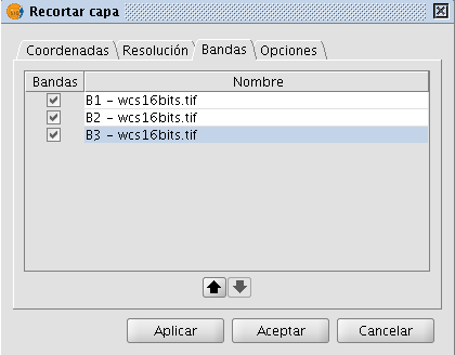
Band selection
The "Bands selection" tab of the Clipping dialog displays a table that lists the bands of the input image. When processed, the output image will have the bands in the order as shown in this list. By default, the output image will have the same order of bands as the input image. The order of the bands can be modified through the "Up" and "Down" buttons. The selected row will go up or down one position in the list. The bands can also be omitted from the resulting image by un-checking the corresponding row.
Clipping dialog. Bands selection tab
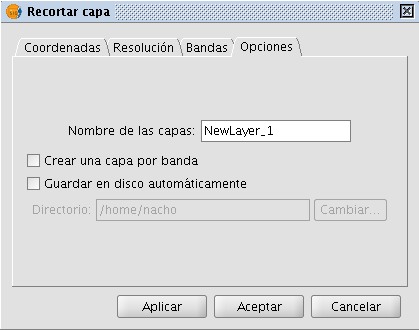
Selecting Options
The "Options" tab of the Clipping dialog presents various options that can be set by the user:
- Name of the output layer: you can modify the default name in the textbox labeled "Layer names". This is the name that will appear in the TOC and the name of the file that will be saved to disk. In case of several output layers (i.e. when each band is saved as a separate layer), the name will be the same for each layer but with a number at the end (_XXX). For example, if the layer is called NewLayer and there are 3 output layers, the respective layer names will be NewLayer_1.tif, NewLayer_2.tif and NewLayer_3.tif.
- If the check box labeled as "Create a layer for each band" is ticked, a new layer will be created for each band in the input image.
- If the check box labeled as "Save on disk automatically" is ticked, a text box labeled "Directory" will be activated where you can indicate the file path for the output files. If un-checked, the generated output layers are temporary.
Clipping dialog. Options tab
Zoom to raster resolution
You can zoom to raster resolution by right-clicking on the layer in the TOC. In the context menu that appears, click "Zoom to raster resolution".
This will activate a crosshair cursor in the gvSIG view which allows users to perform an action by clicking somewhere in the view. The action in this case is that with every mouse-click, the view will be centered on the point where you clicked. In addition, the view will zoom so that one screen pixel is the same size as a pixel in the current raster layer.
Automatic vectorization
The "automatic vectorization" function can be launched from the raster toolbar by selecting "Raster process" on the left drop-down button and "Vectorization" on the drop-down button on the right. Make sure that the name of the raster layer that you want to vectorize is displayed as current layer in the text box.

Vectorization icon
With automatic vectorization, you can generate a vector layer from a raster image using preprocessing to highlight the features of interest.
When launching the Vectorization dialog, the first step is to select the area of the image that you want to vectorize. Keep in mind that the vectorization process may take a long time, so it is recommended to minimize the area (number of pixels) for vectorization. The selection of the area for vectorization can be done in several ways. You can type the coordinates directly; either in pixel coordinates or in the map coordinates. The area can also be selected from the view by clicking the button "Select from the view", after which you can draw an approximate rectangle to define the area. Another selection option is by Region Of Interest (ROI). You can define a ROI here or use a previously defined ROI to set the area for vectorization. In the section "ROI selection" appears a list of available ROI and a checkbox next to each of these to select one or more ROI that you want to use. There are two options to vectorize the ROI: to vectorize the entire area inside the rectangle (bounding box) that covers all the selected ROI, or vectorize only the areas inside the ROI while considering the values outside the ROI as NoData values, excluding them from the calculations.
Finally you can select the scale of the image to preprocess. This is useful because a higher resolution of the preprocessed image will result in a higher precision for the resulting vector layer. You can define this with the drop-down text box labelled "Output Scale". By default, the resolution will be the same as the input image.
When moving on to the next step of the wizard, the process of cutting the image for preprocessing is started. A progress bar appears with the warning that this operation could take a few minutes. The resulting image cut is saved in the temporary folder of gvSIG.

Vectorization. Selection of the area to vectorize
There are two methods to preprocess a raster image to vectorize. The first is by creating a limited number of grayscale levels from the original image. The image will be converted to grayscale using one single band or a combination of bands (use the drop-down button labelled "Bands"). For the conversion to grayscale, a posterization process is used to reduce the number of different values. (By default, the image is reduced into 2 levels only: black and white.) For this process you can control the threshold on which the values are passing from black to white and vice versa. This can be done by moving the "Treshold" slider while you can see a preview of the result. (The Treshold slider is only available when there are 2 levels; when there are intermediate grayscale levels, the slider is disabled.) In addition to the posterization threshold, you can apply a mode filter or a noise filter to smoothen the result.

Vectorization. Conversion to grayscale
The second preprocessing method is useful to vectorize contour lines and can be applied to data types other than byte. With this method you can define intervals between each contour line to be vectorized. You can specify the number of intervals in which you want to divide the raster, or indicate the size of each interval. The cuts that have been selected will be shown on a graph that represents the histogram of the image. On this graph, you can modify the distance between cuts, or add or remove some of them using the mouse. It is also possible to modify the distance between cuts in numeric format using the table on the right of the histogram. Each entry in the table represents a cut with the corresponding value. This type of preprocessing is used for digital elevation models (for example .adf or .asc images).
When moving on to the last step of the vectorization wizard, the preprocessed image is generated with the specified values, and saved in the temporary directory of gvSIG.

Vectorization. Define intervals for vectorization in case of Digital Elevation Models
The last step is to select the method for generation of vectors. There are two methods: contour and potrace, that can be selected from the drop-down button after which a panel appears with settings that are specific for the method. The first method is the simplest and does not have any options. This method will trace the vectors in straight sections going through the pixel centers. This generates a network of vectors based on very small straight sections. The potrace method uses the potrace library for vectorization. The available options for this method are those that the potrace library provides and they are used to define the precision of the tracing of the curves: number of points for each curve, threshold, optimization, etc.

Vectorization. Options for vector generation
When clicking on "Apply" or "Accept", the process of vectorization will start after which you will be prompted whether to display the generated layer in the TOC.
Analysis view
The "Analysis view" can be launched from the raster toolbar by selecting "Raster layer" from the left drop-down button and "Analysis View" on the drop-down button on the right. Make sure that the name of the raster layer that you want to analyze is displayed as current layer in the text box.

Analysis View icon
With this functionality you can zoom in on the current raster layer with 3 different zoom levels:
- On the left of the view, the layer is added to the locator map of gvSIG. This provides a general view of the layer, and you can zoom into the locator map by clicking and dragging, thus drawing a red rectangle. The area inside the red rectangle will be displayed in the view.
- The view itself is the second zoom level which functions independently, and the zoom variations that are performed on the view will be applied to the locator map as well so that it keeps being centered on the correct area.
- When launching the Analysis view, a small floating window labelled "Cursor Zoom" appears in the upper right corner of gvSIG. This window has the highest zoom level. The zoom level is fixed and always centered on the mouse point. By moving the mouse over the gvSIG view, you will see the contents change.
You can change the relation between the zoom level of this floating window and the gvSIG view. This is done by right-clicking on the floating window and selecting one of the values that are shown in the drop-down menu that appears. The available options are x4, x8, x16, and x32. This means that the pixels in the floating window will be 4, 8, 16, or 32 times bigger than the original.
The floating window also shows the RGB values of the pixel on which the cursor is currently located. The text colour of the RGB values as well as the colour of the central cross (red by default) can be changed by right-clicking on the floating window and choosing the option from the drop-down menu.
Keep in mind that, to see the effects in the floating window while moving the mouse over the view, the view must be active. If it is not active, just click on the view. When the cursor is outside the view, the content of the floating window appears black.
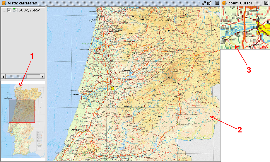
Screenshot with the different elements of Analysis View
There can only be one Analysis view open at any time in gvSIG. Therefore, the button "Analysis View" is re-labelled as "Close Analysis View" when the Analysis view is already open, so that it can be closed before re-opening.
